
AI-generated illustration created to represent the article’s subject. It does not depict an actual EPW course, trainer, participant, client, event or venue.
A time series forecast is useful only when it arrives at the right horizon, at the right level of detail and with enough evidence for someone to act. A lower error score is not automatically a better business forecast. It may conceal leakage, perform poorly during peaks or predict a quantity that does not match the real planning decision.
This article explains an eight-step time series forecasting process using EPW’s FORECAST framework. It covers the full path from decision framing and simple baselines to temporal validation, uncertainty, deployment and monitoring. The process applies whether the final model is statistical, tree-based, neural or an ensemble.
Why time series forecasting needs a different process
Ordinary supervised-learning workflows often assume that examples can be shuffled. Time series data cannot. Order carries information, and future observations must not influence a model evaluated on the past. Scikit-learn’s official guidance warns that standard cross-validation can train on future data and evaluate on earlier data; its TimeSeriesSplit preserves order through expanding training windows.
Forecasting also introduces decisions that a generic prediction project may not face:
- How far ahead must the forecast extend?
- At what frequency and organisational level is it required?
- Which values will actually be known at forecast time?
- How should seasonality, promotions, closures or structural breaks be represented?
- Does the decision need a point estimate, a range or a scenario?
The answer changes the dataset, validation design, metrics and operational value. A one-day staffing forecast and a twelve-month capital forecast are not the same modelling problem, even if both predict demand.
The EPW FORECAST process
FORECAST is an eight-stage workflow for producing forecasts that remain honest about time and useful for decisions.
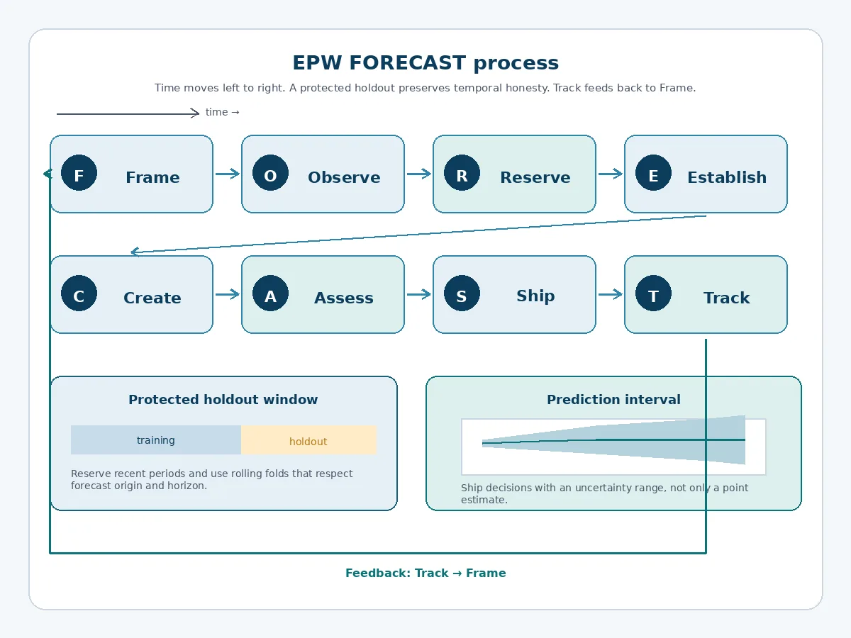
1. Frame the decision, horizon and granularity
Begin with the action. Identify who uses the forecast, what they decide, when they decide it and what can still be changed. Then define the forecast origin, horizon, frequency and granularity. “Forecast sales” is incomplete; “each Monday, forecast the next six weeks of unit demand by distribution centre for replenishment planning” is testable.
Record operational constraints such as minimum order quantities, staffing lead times or storage capacity. A forecast at a finer level can be harder to estimate and may not improve the decision. Use the lowest granularity that creates meaningful action, not the finest data available.
2. Observe the data-generating process
Plot the series before choosing a model. Examine trend, multiple seasonal cycles, calendar effects, intermittent demand, outliers, missing intervals and changes in variance. Distinguish a true zero from an unrecorded value. Mark policy changes, launches, closures, supply constraints and measurement changes.
Ask how each observation was produced. Recorded sales may be lower than demand when stock was unavailable. Call volumes may reflect a system outage rather than normal customer behaviour. Treating a constrained or changed process as stable history can teach the model the wrong pattern.
3. Reserve temporal test windows
Create the evaluation design before feature engineering or tuning. Keep the latest suitable period as a final holdout, then use rolling-origin or expanding-window validation inside the earlier data. Each fold should reproduce the information boundary and forecast horizon expected in production.
Add a gap when recent features could leak information across the split, and ensure transformations are fitted only on each training window. Include enough folds to cover normal and difficult periods. A single calm month is weak evidence for a model that must handle annual peaks.
4. Establish simple and operational baselines
Simple forecasts are essential controls. Depending on the series, compare the last observed value, seasonal naïve forecast, historical average or a basic trend. The online textbook Forecasting: Principles and Practice emphasises that simple methods can be surprisingly effective benchmarks.
Also include the current organisational method, such as a planner’s spreadsheet or vendor forecast. A complex model must beat a relevant baseline by enough to justify data engineering, compute, monitoring and change. If it cannot, keep the simpler method and investigate the problem definition.
5. Create valid features and candidate models
Build lagged values, rolling summaries and calendar features using information available at the forecast origin. External predictors such as price, weather or planned campaigns are valid only if their future values are known or separately forecast. A realised future promotion value is leakage when planners would possess only a plan.
Compare model families rather than assuming machine learning must win. Statistical methods can represent level, trend and seasonality clearly. Tree-based models can exploit nonlinear relationships across lag and external features. Recurrent or transformer-based methods may help with large panels or complex sequences but require stronger evidence and resources. Ensembling can improve robustness when component errors differ.
6. Assess error, uncertainty and decision impact
Choose metrics based on consequences. Mean absolute error is interpretable in original units; root mean squared error places more weight on large errors. Percentage measures can become unstable around zero, while aggregate weighted measures can hide weak performance on small but important series.
Report performance by horizon, season, location and demand pattern. Compare forecast bias because persistent under-forecasting and over-forecasting create different costs. Where decisions depend on risk, provide prediction intervals or quantiles and check their empirical coverage. An interval that claims 90% coverage should contain the realised outcome at approximately that rate under comparable conditions.
7. Ship forecasts into a controlled decision
Define the production schedule, data cut-off, model version, output schema and fallback. Present the forecast with its horizon, uncertainty, recent error and relevant drivers or events. Let users record overrides and reasons; do not overwrite the original forecast, because that destroys the evidence needed to evaluate judgement.
Test the end-to-end workflow. A model that runs after the planning meeting or produces product codes that do not map to the ordering system has no operational value. Confirm that recipients, approvals and exception queues work before scaling.
8. Track forecast and outcome performance
Monitor data arrival, missingness, feature distributions, forecast error, bias, interval coverage, overrides and business outcomes. Use a maturity period appropriate to the horizon: a six-month forecast cannot be fully judged next week. Separate model degradation from process changes such as altered prices or capacity.
Define thresholds and actions in advance. The response might be investigation, temporary baseline fallback, retraining, recalibration or retirement. Monitoring should also test whether the forecast improves the downstream decision rather than merely whether its values look plausible.
Worked example: weekly support-demand planning
A service centre schedules specialist staff four weeks ahead. It has three years of daily contact volumes, event dates, planned product releases and staff calendars. The decision is how many specialist shifts to schedule by week, subject to minimum staffing and overtime limits.
The team applies FORECAST as follows:
- Frame: produce four weekly forecasts every Monday at service-line level.
- Observe: identify weekday patterns, year-end peaks, launch spikes and missing records during one platform outage.
- Reserve: hold out the latest twelve weeks and run rolling four-week backtests across the preceding year.
- Establish: compare seasonal naïve, the planners’ existing method and a regularised regression baseline.
- Create: test calendar, lag, rolling-volume and known launch-plan features in tree-based and statistical candidates.
- Assess: review MAE, peak-week bias and 80% interval coverage by horizon and service line.
- Ship: convert quantile forecasts into base staffing plus an exception queue for uncertain peaks.
- Track: monitor forecast error, overtime, service level and planner overrides.
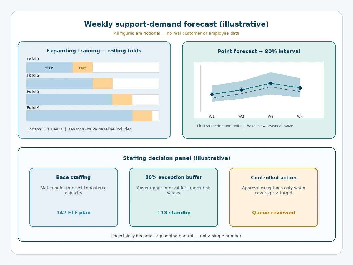
Suppose the tree-based model lowers average error but under-forecasts the busiest launch weeks. The planners may prefer an ensemble with slightly higher overall MAE but better peak bias and interval coverage. That is a rational selection because the cost of understaffing peaks dominates small improvements during normal weeks.
Forecast evaluation scorecard
| Evidence layer | Questions | Example measures |
|---|---|---|
| Temporal validity | Did every test reproduce the information available at the forecast origin? | Rolling folds, gap, horizon match, leakage checks |
| Point accuracy | How large are typical and costly errors? | MAE, RMSE, WAPE, horizon-specific error |
| Uncertainty | Are ranges informative and calibrated? | Interval width, quantile loss, empirical coverage |
| Operational use | Did users receive and apply the forecast in time? | Delivery rate, override rate, exception resolution |
| Business outcome | Did the decision improve without unacceptable side effects? | Service level, overtime, stock-outs, waste or delay |
Time series forecasting checklist
- Is the decision owner, forecast origin, horizon, frequency and granularity documented?
- Have zeros, missing intervals, outliers and structural breaks been investigated?
- Does the validation scheme preserve time and reproduce the production horizon?
- Are simple, seasonal and current operational baselines included?
- Were all lags, rolling features and transformations calculated without future information?
- Will external predictors be known at forecast time?
- Are error, bias and uncertainty reviewed across horizons and important segments?
- Can users see assumptions, record overrides and fall back safely?
- Are monitoring triggers linked to named corrective actions?
- Is downstream decision value measured separately from model accuracy?
Develop a complete forecasting capability
Reliable forecasting requires more than fitting algorithms. Teams need judgement about time boundaries, data-generating processes, baselines, backtesting, uncertainty and workflow design. EPW’s Time Series Forecasting with Machine Learning Methods Course develops these capabilities through preprocessing, feature engineering, model comparison, evaluation and an end-to-end forecasting project.
For wider context on selecting AI investments, read Benefits of AI and Machine Learning for Organisations. The strongest forecast is not simply the model with the smallest headline error. It is the forecast that uses honest temporal evidence and improves a real decision within known uncertainty.
References
- Scikit-learn, TimeSeriesSplit documentation, version 1.9; accessed 4 September 2026.
- Hyndman, R. J. and Athanasopoulos, G., Forecasting: Principles and Practice, third edition; accessed 4 September 2026.
- Scikit-learn, Lagged features for time series forecasting, accessed 4 September 2026.
- EPW Training, Time Series Forecasting with Machine Learning Methods Course, accessed 4 September 2026.