

AI-generated illustration created to represent the article’s subject. It does not depict an actual EPW course, trainer, participant, client, event or venue.
A PV loss tree converts the gap between available solar resource and delivered electrical energy into traceable loss categories, while performance ratio (PR) expresses the plant’s final yield relative to its reference yield. Used together, they help photovoltaic designers, performance engineers, asset managers and lenders distinguish normal conversion losses from data errors, equipment underperformance and avoidable operational losses.
This article presents a reusable model for expected-yield studies and operating-plant analysis. It explains the calculation boundary, the correct sequence of losses, a completed illustrative example, interpretation rules and the evidence needed before an engineer recommends corrective work.
What the PV loss-tree and performance-ratio model measures
A loss tree is a reconciled energy pathway. It begins with a defined reference energy and applies losses in the physical order in which they occur. The result should match the modelled or measured energy at the delivery boundary. A performance ratio is a normalised indicator, so it makes performance more comparable across periods with different irradiation.
These are related but different tools. The loss tree explains where energy is lost. PR summarises how effectively the plant converts the available in-plane irradiation into usable output. The PVsyst performance-ratio documentation identifies optical, array and system losses within this relationship. The IEA Photovoltaic Power Systems Programme Task 13 also treats performance, durability and reliability as connected technical and economic concerns.
1. Define boundaries and energy terms
Write the boundary before calculating any percentage. State whether the output is measured at inverter alternating-current terminals, the low-voltage collection system, the point of connection or the revenue meter. Also state whether transformer consumption, station service, export limitation and battery charging sit inside or outside the model.
Use consistent terms:
- Plane-of-array irradiation is the solar energy received on the module plane over the assessment period.
- Reference yield normalises plane-of-array irradiation by the reference irradiance used for the rated array power.
- Array yield relates direct-current energy from the array to installed direct-current capacity.
- Final yield relates delivered alternating-current energy to installed reference capacity.
- Performance ratio is final yield divided by reference yield for the same period and boundary.
Document the capacity basis. A direct-current module nameplate basis and an alternating-current inverter basis produce different interpretations. Record sensor class, calibration status, data interval, missing-data treatment, curtailment flag and time zone. A loss calculation is not reliable if its irradiation and energy timestamps are misaligned.
2. Build the PV loss tree in physical order
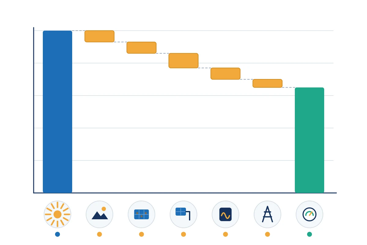
Begin with modelled reference energy and apply each loss sequentially. Percentages must not simply be added when each acts on the remaining energy. Group the loss tree into four levels so reviewers can test the assumptions.
| Loss level | Typical categories | Evidence |
|---|---|---|
| Solar resource and geometry | Transposition, horizon, near shading, incidence-angle effects | Meteorological source, site survey, layout and shading model |
| Optical and module environment | Soiling, snow where relevant, spectral effects and irradiance variation | Soiling stations, cleaning records, climate data and module response model |
| Direct-current array | Temperature, module quality, mismatch, degradation and DC wiring | Module files, thermal model, test data, string monitoring and cable design |
| Conversion and delivery | Inverter efficiency, clipping, availability, transformer, auxiliary and grid losses | Inverter curves, alarms, outage logs, meter data and electrical studies |
Keep forced losses separate from controllable losses. For example, temperature loss arises from operating conditions and module characteristics, while avoidable inverter downtime may be an operational issue. Curtailment should normally be reported separately from conversion performance because it may be caused by a grid instruction or commercial constraint rather than equipment inefficiency.
Maintain a loss dictionary. Each category needs a definition, calculation method, data source, owner and rule preventing double counting. If measured availability already captures an inverter outage, do not also apply the same lost energy as a generic operational adjustment.
3. Calculate performance ratio on a consistent basis
The common relationship is:
PR = final yield ÷ reference yield
Equivalently, final yield is delivered energy divided by installed reference power, while reference yield is plane-of-array irradiation divided by reference irradiance. Use compatible units throughout. The performance ratio is dimensionless and is usually expressed as a percentage.
PR is not the same as capacity factor. Capacity factor compares energy with the output that would occur if rated power were sustained for every hour. PR instead normalises output for the solar resource received. It is also not a direct efficiency measurement: installed capacity, irradiation measurement, temperature and system boundary all influence it.
Weather-corrected PR can help compare periods, but every correction method must be declared. Do not compare a temperature-corrected contractual PR with an uncorrected operational dashboard value. The US Department of Energy’s Understanding Solar Photovoltaic System Performance illustrates how measured and modelled performance indicators depend on analysis assumptions and data quality.
4. Complete an illustrative loss-tree model
Assume an illustrative study begins with 1,000 MWh of reference energy for the selected period. The following figures demonstrate the calculation method only; they are not benchmarks for a real plant.
| Stage | Loss applied | Energy remaining |
|---|---|---|
| Reference energy | — | 1,000.0 MWh |
| Soiling | 3.0% | 970.0 MWh |
| Shading and incidence effects | 2.0% | 950.6 MWh |
| Mismatch and DC wiring | 2.5% | 926.8 MWh |
| Temperature and module operation | 3.0% | 899.0 MWh |
| Inverter conversion and clipping | 1.5% | 885.6 MWh |
| Availability and delivery | 1.0% | 876.7 MWh |
The combined loss is 12.3%, not the simple 13.0% sum of the individual percentages, because each loss is applied to the remaining energy. On a consistent capacity and irradiation basis, the example corresponds to a PR of approximately 87.7%.
Now suppose the meter records 850 MWh after validated exclusions. The unexplained gap is 26.7 MWh. The team should not create a new “miscellaneous loss” and close the analysis. It should test hypotheses: underestimated soiling, additional curtailment, inaccurate irradiation, temperature-model error, string outages, inverter derating, meter scaling or timestamp mismatch.
A completed model therefore contains both the loss waterfall and an uncertainty band. If expected energy is 876.7 MWh with a justified uncertainty range, the significance of an 850 MWh result depends on that range. A small variance inside measurement and modelling uncertainty calls for monitoring; a persistent variance outside it calls for diagnosis.
5. Interpret differences without false precision
Use three tests before assigning a cause:
- Materiality: Is the energy gap large enough to change an operational or financial decision?
- Persistence: Does it remain after data-quality checks and across comparable periods?
- Localisation: Can it be associated with a subsystem, operating state, weather condition or alarm pattern?
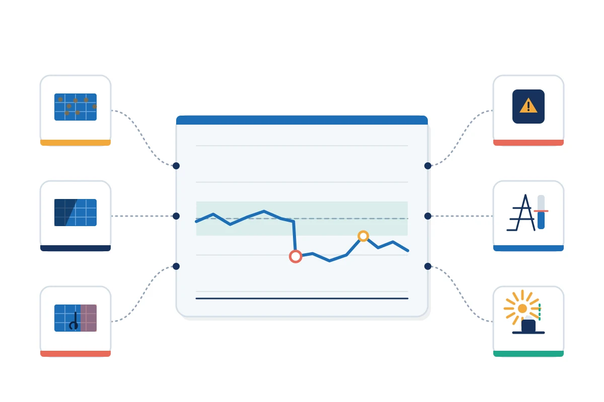
Analyse daily or sub-daily residuals as well as the annual total. A midday residual may indicate clipping, temperature or export limitation. A morning and evening pattern can point to shading or horizon assumptions. A step change may align with an outage, firmware change, meter replacement or sensor drift.
For long-term trends, avoid fitting a degradation rate to untreated raw energy. The IEA PVPS assessment of performance-loss-rate methods explains that different calculation approaches can produce inconsistent results and that power and weather data require suitable filtering and treatment. Record the method, filters, minimum period and confidence interval.
6. Use the model in design and operation
During design, the model makes the energy estimate auditable. Independent reviewers can test the irradiation source, layout, component assumptions, availability and grid constraints. PVWatts provides a transparent route for preliminary grid-connected PV energy estimates, while detailed design normally requires site-specific models and engineering evidence.
During operation, replace assumptions with measured evidence in a controlled order. Update availability from alarms and work orders, reconcile revenue and supervisory-control meters, calculate soiling from paired sensors or cleaning tests, and investigate string or inverter deviations. Keep the original financial baseline separate from the current operational forecast so that the team can explain both variance from plan and expected future production.
The June 2026 IEA PVPS report on photovoltaic project decisions links quality management, monitoring, technical key performance indicators and economic value across the project lifecycle. That lifecycle view is important: correcting an input does not merely improve a chart; it can change maintenance priority, revenue forecasting and investment decisions.
Advantages and limitations
The model is transparent, reviewable and useful for prioritising investigation. It also creates a common language between designers, operators and commercial teams. However, one annual PR value can conceal seasonal faults, curtailment, sensor drift and availability patterns. A loss tree can also appear more certain than its inputs justify.
Do not use PR alone to compare plants with different climates, technologies, boundaries or correction methods. Pair it with specific yield, availability, curtailment, degradation, inverter and string indicators. Preserve raw data and calculation versions so that a future analyst can reproduce the result.
PV loss-tree implementation checklist
- Define the meter boundary and capacity basis.
- Validate irradiation, energy, time stamps and missing-data rules.
- Apply losses sequentially in physical order.
- Separate resource, technical, availability and curtailment effects.
- Prevent overlap through a controlled loss dictionary.
- Calculate PR with consistent units and correction methods.
- Reconcile expected energy with the selected meter.
- Quantify uncertainty before declaring underperformance.
- Use residual patterns to test causes.
- Version the model and retain the original baseline.
Conclusion
A useful PV loss tree is more than a list of percentages. It is a reconciled model in which every material loss has a definition, position, source and owner. Performance ratio then provides a compact normalised result. Together, the two tools turn an energy shortfall into a structured engineering investigation while keeping uncertainty and commercial boundaries visible.
Develop practical photovoltaic analysis skills
EPW’s Photovoltaic System Design and Performance Analysis course develops the engineering judgement needed to evaluate resource data, system losses, yield models and operating results. Explore related programmes in the Electrical Power and Energy Engineering category.
Sources and References
- International Energy Agency Photovoltaic Power Systems Programme. Task 13: Performance, Operation and Reliability of Photovoltaic Systems.
- International Energy Agency Photovoltaic Power Systems Programme. Assessment of Performance Loss Rate of PV Power Systems. 2021.
- International Energy Agency Photovoltaic Power Systems Programme. Photovoltaic Project Decisions: Quality, Performance, and Economic Value. June 2026.
- US Department of Energy. Understanding Solar Photovoltaic System Performance. 2022.
- PVWatts. PVWatts Calculator.
- PVsyst. Performance Ratio.