
AI-generated illustration created to represent the article’s subject. It does not depict an actual EPW course, trainer, participant, client, event or venue.
Most business datasets are presented as rows, yet many important problems are really about relationships. A payment connects an account to a merchant. A component belongs to an asset and depends on other components. A shipment links a supplier, route, port and customer. Graph neural networks (GNNs) are designed for this connected structure.
This guide explains how GNNs work, compares the main architecture families and shows how to decide whether they are justified. The goal is not to select the newest model. It is to connect a clearly defined decision to a defensible graph, an appropriate learning task and a realistic evaluation design.
What is a graph neural network?
A graph contains nodes, which represent entities, and edges, which represent relationships. Nodes and edges may both carry features. In a maintenance graph, nodes might be pumps, motors and valves; an edge might record physical connection, functional dependency or shared operating context.
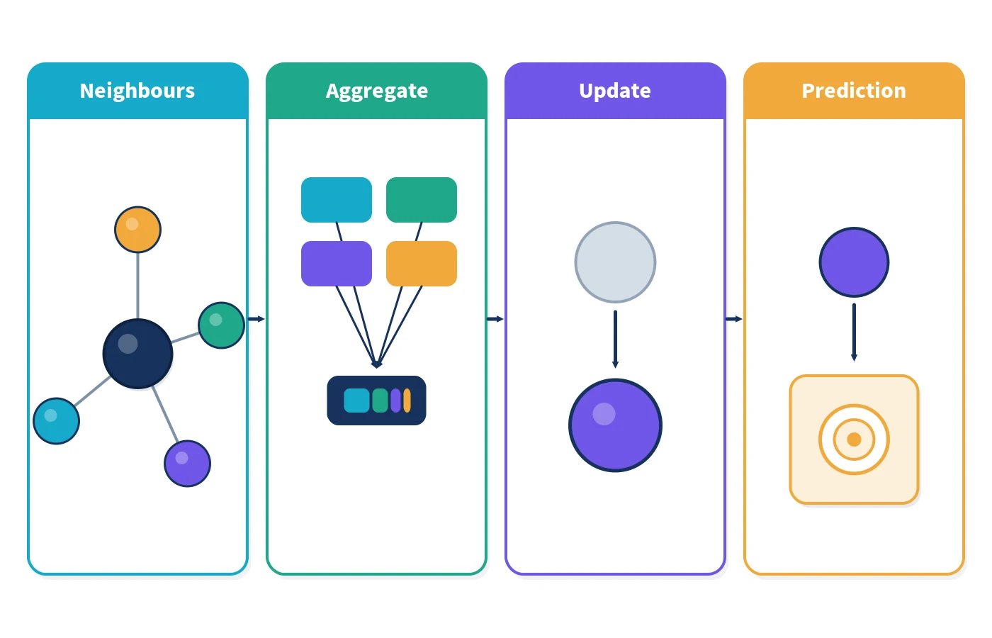
A GNN transforms this structure into useful representations. Most common GNN layers use message passing: each node receives information from selected neighbours, aggregates it and updates its own representation. The official PyTorch Geometric documentation expresses this through message, aggregation and update functions. Stacking layers lets information travel farther, although more layers are not automatically better.
The output depends on the task:
- Node classification: label an account as high risk, a machine as likely to fail or a document as belonging to a category.
- Link prediction: estimate whether two entities should be connected, such as a likely supplier relationship or product interaction.
- Graph classification: classify an entire graph, such as a molecular structure, transaction subgraph or process network.
- Graph regression: estimate a continuous value for a whole network or subgraph.
How message passing works
Imagine a node representing one supplier. Its own features include location, lead-time history and quality performance. Its neighbours include parts, plants and logistics providers. A message-passing layer combines selected neighbour information with the supplier’s current representation. After one layer, the node represents its immediate context; after two, it may incorporate neighbours of neighbours.
This is powerful because two suppliers with similar individual records may pose different risks when one sits inside a fragile dependency network. It is also risky: an incorrect edge definition can spread misleading information. The graph is part of the model, not a neutral container.
Main types of graph neural network
| Architecture | Core idea | Useful when | Watch for |
|---|---|---|---|
| Graph Convolutional Network (GCN) | Applies normalised neighbourhood aggregation | You need a strong, relatively simple baseline on a mostly homogeneous graph | Repeated smoothing can make node representations too similar |
| GraphSAGE | Samples neighbours and learns an aggregation function | The graph is large or new nodes must be handled | Sampling policy can omit important context |
| Graph Attention Network (GAT) | Learns different weights for neighbours | Neighbour relevance is unequal and learned weighting may help | Attention adds cost and is not automatically an explanation |
| Relational or heterogeneous GNN | Uses different transformations for node or edge types | The graph contains materially different entities and relationship semantics | Many types increase parameters, data needs and governance effort |
| Temporal GNN | Models relationships and events that change over time | Order, recency or network evolution affects the target | Future information can leak into training if time is mishandled |
| Graph autoencoder | Learns compressed graph representations, often by reconstructing links | You need embeddings, anomaly signals or unsupervised structure learning | A plausible reconstruction may not align with the business outcome |
The original GCN paper by Kipf and Welling described an efficient convolutional approach that encodes local graph structure and node features. GraphSAGE introduced an inductive method that samples and aggregates neighbours so representations can be generated for unseen nodes. Graph Attention Networks allowed a model to assign different learned weights to neighbours. These are design patterns, not a ranking: the best choice depends on the task, graph dynamics and operating constraints.
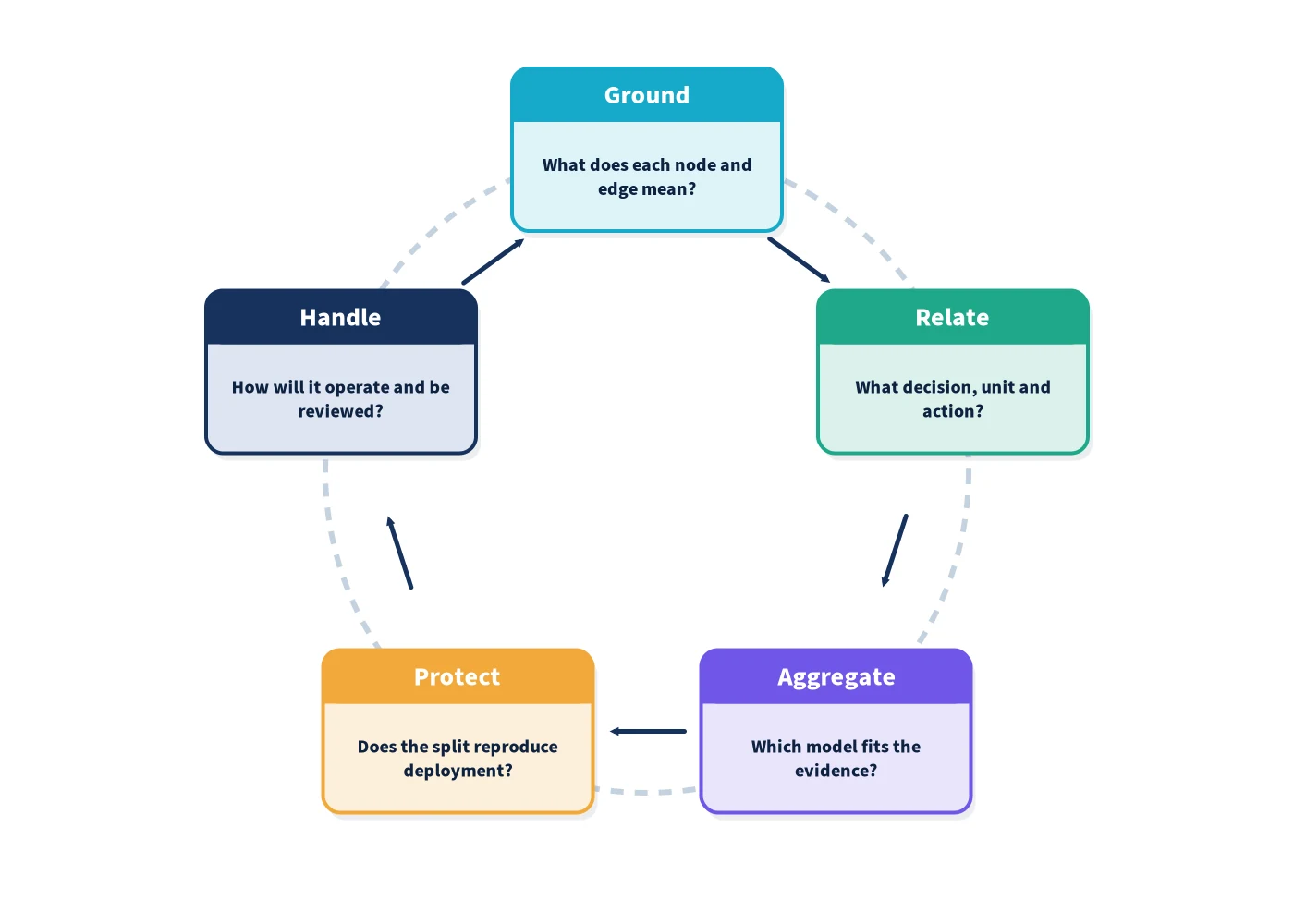
The EPW GRAPH design framework
Use the following five-stage framework before choosing an architecture.
G — Ground the graph
Define what each node and edge means. State whether edges are directed, weighted, signed or time-stamped. Decide whether absence of an edge means “no relationship”, “unknown” or merely “not yet observed”. Record how identities are resolved and how duplicate entities are handled. A graph with ambiguous semantics produces ambiguous learning.
R — Relate the graph to the decision
Write the operational decision, prediction unit and action. “Identify risky nodes” is incomplete. “Rank supplier sites each week for resilience review, using only information available at the weekly cut-off” is testable. Select node, link or graph prediction only after this statement is clear.
A — Aggregate appropriately
Start with a transparent baseline: node features alone, a simple network statistic or both. Then compare a modest GCN or GraphSAGE model. Add attention, relationship-specific parameters or temporal components only when the graph and evaluation evidence support them. Choose the neighbourhood depth using domain logic; two hops in a supply chain may mean something very different from two hops in a social network.
P — Protect the evaluation
Randomly splitting nodes or edges can leak connected information across train and test sets. Use time-based, entity-based or graph-based splits that reproduce deployment. The Open Graph Benchmark provides task-specific data loaders, splits and evaluators for realistic graph-learning research; its design is a useful reminder that the split is part of the problem definition.
H — Handle operation and human review
Specify inference frequency, latency, memory and graph-refresh requirements. Monitor feature drift, degree distribution, new node types, missing edges and performance by relevant group. Give reviewers the evidence they need, such as influential paths or neighbouring events, while making clear that attention weights or saliency scores do not prove causation.
Worked example: supply-network disruption risk
Consider a manufacturer that wants to prioritise supplier reviews. Nodes represent supplier sites, parts, plants and transport hubs. Typed edges represent “supplies”, “used by” and “moves through”. Features include delivery variability, capacity, quality events and lead times. The target is whether a supplier site contributes to a material disruption in the next 30 days.
- Baseline: train a tabular model using supplier-site features and compare it with rules based on late deliveries and single-source status.
- Graph model: use a relational GNN so that supply and transport edges have different meanings. Limit messages to information available at the weekly cut-off.
- Split: train on earlier periods and test on later periods. Hold out selected suppliers to test generalisation to new sites.
- Metrics: measure precision among the top review candidates, recall of subsequent disruptions, calibration and lead time. Report results by supplier region and category.
- Operation: present risk as a review priority, not proof that a supplier caused a disruption. Require planners to record the action and outcome.
If the GNN does not materially improve decision-relevant performance over the baseline, the simpler model may be the better production choice. Relationship data creates value only when it changes the decision reliably enough to justify its cost.
When a GNN is—and is not—the right choice
A GNN is promising when relationships are stable enough to model, neighbouring context carries predictive information, and the task naturally concerns nodes, links or complete graphs. It is less attractive when edges are unreliable, the dataset is small, the target depends mostly on individual attributes or a conventional model already meets the operational need.
Also test graph-free alternatives. Add network statistics—degree, centrality, community or counts of risky neighbours—to a tabular model. This often reveals whether structural information helps before a complex architecture is introduced.
Practical GNN checklist
- Can every node and edge type be defined in plain language?
- Does the graph reflect the information available at prediction time?
- Is the task node, link or graph prediction?
- What non-GNN baseline must the model beat?
- Does the split prevent temporal and relational leakage?
- How will unseen nodes and changing relationships be handled?
- Which errors matter operationally, and for whom?
- Can the graph be refreshed, versioned and audited?
- What monitoring signals will trigger investigation or retraining?
Governance questions specific to connected data
Graph projects introduce governance issues that a row-based workflow can obscure. One person’s record may affect another node’s prediction through shared neighbours. Teams should document whether those inferred relationships are permitted, relevant and proportionate. They should also distinguish a directly observed link from an inferred one and preserve its provenance.
Access control deserves particular attention. A user who cannot see a sensitive node should not receive an explanation that reveals its presence through a path or neighbourhood summary. Apply privacy and security tests to graph extracts, embeddings, caches and explanation artefacts—not only to the source tables. Where relationships are commercially sensitive, use the minimum subgraph needed for the task and define retention rules.
Finally, record model limitations in operational language. A fraud GNN may identify unusual connectivity without proving wrongdoing; a supply-network model may surface concentration risk without knowing an undisclosed supplier. Human reviewers need this boundary, the data cut-off and the reason a case was prioritised. These controls make the model’s relational advantage usable without turning correlation into an unsupported conclusion.
Build graph-learning capability around decisions
Graph neural networks are most useful when a team understands both network structure and machine-learning discipline. EPW’s Graph Neural Networks and Network Analysis course covers graph theory, message passing, GCNs, attention, network analysis, practical tools and real-world solution design. It connects naturally with EPW’s wider guidance on the benefits of AI and machine learning for organisations.
The durable lesson is simple: start with the relationship and decision, not the architecture name. Ground the graph, test a baseline, protect the evaluation and plan for operation. A well-designed graph model can reveal context that rows conceal; a poorly designed one can spread error through every connection.